
ファイル:Hamiltonian flow classical.gif
高解像度版はありません。
Hamiltonian_flow_classical.gif (195 × 390 ピクセル、ファイルサイズ: 172キロバイト、MIME タイプ: image/gif、ループします、86 フレーム、26秒)
ウィキメディア・コモンズのファイルページにある説明を、以下に表示します。
|
概要
| 解説 |
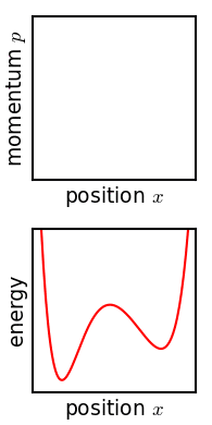
English: Flow of a statistical ensemble in the potential x**6 + 4*x**3 - 5*x**2 - 4*x. Over long times it becomes swirled up, and appears to become a smooth and stable distribution. However, this stability is an artifact of the pixelization (the actual structure is too fine to perceive). This animation is inspired by a discussion of Gibbs in his 1902 wikisource:Elementary Principles in Statistical Mechanics, Chapter XII, p. 143: "Tendency in an ensemble of isolated systems toward a state of statistical equilibrium". A quantum version of this can be found at File:Hamiltonian flow quantum.webm |
| 日付 | |
| 原典 | 投稿者自身による著作物 |
| 作者 | Nanite |
Source
この GIF ラスター画像はMatplotlibで作成されました。
この 画像はImageMagickで作成されました。
Python source code. Requires matplotlib ImageMagick. Possibly does not run in Windows.
from pylab import *
import subprocess
import sys
import os

figformat = '.png'
seterr(divide='ignore')
rcParams['font.size'] = 9

#define color map that is transparent for low values, and dark blue for high values.
# weighted to show low probabilities well
cdic = {'red':   [(0,0,0),(1,0,0)],
        'green': [(0,0,0),(1,0,0)],
        'blue':  [(0,0.7,0.7),(1,0.7,0.7)],
        'alpha': [(0,0,0),
                  (0.1,0.4,0.4),
                  (0.2,0.6,0.6),
                  (0.4,0.8,0.8),
                  (0.6,0.9,0.9),
                  (1,1,1)]}
cm_prob = matplotlib.colors.LinearSegmentedColormap('prob',cdic,N=640)

### System dynamics ###

# potential is a polynomial
potential_coefs = array([1,0,0,4,-5,-4,0],'d')
def potential(x,t):
    return polyval(potential_coefs,x)

# force function is its derivative.
force_coefs = (potential_coefs*arange(len(potential_coefs)-1,-1,-1))[:-1]
def force(x,t):
    """ derivative of potential(x) """
    return polyval(force_coefs,x)
invmass = 1.0
dt = 0.03

def motion(t,x,p):
    """ returns dx/dt, dp/dt """
    return p*invmass, -force(x,t)

cur_x = -0.1
cur_p = 0

def rkky_step(t, x_i, p_i, dt):
    kx1,kp1 = motion(t, x_i, p_i)
    dt2 = 0.5*dt
    kx2,kp2 = motion(t+dt2, x_i+dt2*kx1, p_i+dt2*kp1)
    kx3,kp3 = motion(t+dt2, x_i+dt2*kx2, p_i+dt2*kp2)
    kx4,kp4 = motion(t+dt, x_i+dt*kx3, p_i+dt*kp3)
    newx = x_i + (dt/6.0)*(kx1 + 2.0*kx2 + 2.0*kx3 + kx4)
    newp = p_i + (dt/6.0)*(kp1 + 2.0*kp2 + 2.0*kp3 + kp4)
    return newx, newp

### Setup ensemble points ###

# most are randomly chosen
x = 0 + 0.5*rand(20000)
p = -1.0 + 2.0*rand(20000)

# the pilot points are set manually
x[0] = 0;    p[0] = 0
x[1] = 0.4;  p[1] = 0.0
pilots = [0,1]
pilot_colors = {
       0: (0,0.7,0),
       1: (0.7,0,0)}
E = potential(x,0) + 0.5*invmass*p**2

### set up plot limits and histogram bins ###
xedges = linspace(-2.1,1.7,151)
pedges = linspace(-7.5,7.5,151)
Eedges = linspace(-9,9,151)
pix = 150
extent = [xedges[0], xedges[-1], pedges[-1], pedges[0]]
H = histogram2d(x,p,bins=[xedges,pedges])[0].transpose()
cmax = amax(H)*0.8

extenten = [xedges[0], xedges[-1], Eedges[-1], Eedges[0]]
Hen = histogram2d(x,E,bins=[xedges,Eedges])[0].transpose()
cmaxen = amax(Hen)*0.3

fig = figure(1)
ysize = 2.6
xsize = 1.3
fig.set_size_inches(xsize,ysize)

### Prepare lower plot ###
axen = axes((0.2/xsize,0.2/ysize,1.0/xsize,1.0/ysize),frameon=True)
axen.xaxis.set_ticks([])
axen.xaxis.labelpad = 2
axen.yaxis.set_ticks([])
axen.yaxis.labelpad = 2
xlim(-2.1,1.7)
ylim(-9,9)
xlabel('position $x$')
ylabel('energy')
potx = linspace(-2.1,1.7,151)

### Prepare upper plot ###
ax = axes((0.2/xsize,1.5/ysize,1.0/xsize,1.0/ysize),frameon=True)
ax.xaxis.set_ticks([])
ax.xaxis.labelpad = 2
ax.yaxis.set_ticks([])
ax.yaxis.labelpad = 2
xlim(-2.1,1.7)
ylim(-7.5,7.5)
xlabel('position $x$')
ylabel('momentum $p$')

### Start running simulation ###
frames = list()
delays = list()
framemod = 5
frame = "frames/background"+figformat
savefig(frame,dpi=pix)
frames.append(frame)
delays.append(16)

print "generating frames...  0%",
sys.stdout.flush()
savesteps = range(0,401,framemod) + [600, 1000, 2000, 6000]
delays += [10]*len(savesteps)
delays[1] = 200
delays[-5:] = [100,200,200,200,400]
totalsteps = max(savesteps)+1
for step in range(totalsteps):
    if step % 20 == 0:
        print "\b\b\b\b\b{0:3}%".format(int(round(step*100.0/totalsteps))),
        sys.stdout.flush()
    if step in savesteps:
        # Every several frames, do a plot
        remlist = list()

        sca(ax)
        H = histogram2d(x,p,bins=[xedges,pedges])[0].transpose()
        remlist.append(imshow(H, extent=extent, cmap=cm_prob, interpolation='none', aspect='auto'))
        remlist[-1].set_clim(0,cmax)
        for i in pilots:
            remlist += plot(x[i], p[i], '.', color=pilot_colors[i], markersize=3)

        E = potential(x,step*dt) + 0.5*invmass*p**2
        sca(axen)
        pot = potential(potx,step*dt)
        remlist += plot(potx,pot,color='r',zorder=0)
        Hen = histogram2d(x,E,bins=[xedges,Eedges])[0].transpose()
        remlist.append(imshow(Hen, extent=extenten, cmap=cm_prob, interpolation='none', aspect='auto',zorder=1))
        remlist[-1].set_clim(0,cmaxen)
        for i in pilots:
            remlist += plot(x[i], E[i], '.', color=pilot_colors[i], markersize=3)

        frame = "frames/frame"+str(step)+figformat
        savefig(frame,dpi=pix)
        frames.append(frame)
        # Clear out updated stuff.
        for r in remlist: r.remove()
    x, p = rkky_step(step*dt, x, p,dt)
print "\b\b\b\b\b      done"

assert(len(delays) == len(frames))

### Assemble animation using ImageMagick ###
calllist = 'convert -dispose Background'.split()
for delay,frame in zip(delays,frames):
    calllist += ['-delay',str(delay)]
    calllist += [frame]
calllist += '-loop 0 -layers Optimize _animation.gif'.split()
f = open('anim_command.txt','w')
f.write(' '.join(calllist)+'\n')
f.close()

print "composing into animated gif...",
sys.stdout.flush()
subprocess.call(calllist)
print "      done"
os.rename('_animation.gif','animation.gif')
ライセンス
この作品の著作権者である私は、この作品を以下のライセンスで提供します。
| このファイルはクリエイティブ・コモンズ CC0 1.0 全世界 パブリック・ドメイン提供のもとで利用可能にされています。 | |
| ある作品に本コモンズ証を関連づけた者は、その作品について世界全地域において著作権法上認められる、その者が持つすべての権利(その作品に関する権利や隣接する権利を含む。)を、法令上認められる最大限の範囲で放棄して、パブリック・ドメインに提供しています。
この作品は、たとえ営利目的であっても、許可を得ずに複製、改変・翻案、配布、上演・演奏することが出来ます。 |
ファイルの履歴
過去の版のファイルを表示するには、その版の日時をクリックしてください。
| 日付と時刻 | サムネイル | 寸法 | 利用者 | コメント | |
|---|---|---|---|---|---|
| 現在の版 | 2013年10月27日 (日) 08:57 | | 195 × 390 (172キロバイト) | Nanite | Added potential plot (with bonus ensemble histogram in E,x), as well as a couple of "pilot" systems. |
| 2013年10月26日 (土) 22:39 |  | 195 × 195 (84キロバイト) | Nanite | higher resolution + a big longer in time to get the smooth look. | |
| 2013年10月26日 (土) 22:10 |  | 195 × 195 (84キロバイト) | Nanite | User created page with UploadWizard |
ファイルの使用状況
以下のページがこのファイルを使用しています:
グローバルなファイル使用状況
以下に挙げる他のウィキがこの画像を使っています:
- ar.wikipedia.org での使用状況
- ast.wikipedia.org での使用状況
- az.wikipedia.org での使用状況
- en.wikipedia.org での使用状況
- en.wikiversity.org での使用状況
- es.wikipedia.org での使用状況
- fr.wikipedia.org での使用状況
- id.wikipedia.org での使用状況
- pt.wikipedia.org での使用状況
- sl.wikipedia.org での使用状況