
ファイル:Heteroclinic orbit in pendulum phaseportrait.png

このプレビューのサイズ: 800 × 416 ピクセル。 その他の解像度: 320 × 166 ピクセル | 640 × 333 ピクセル | 1,017 × 529 ピクセル。
元のファイル (1,017 × 529 ピクセル、ファイルサイズ: 15キロバイト、MIME タイプ: image/png)
ウィキメディア・コモンズのファイルページにある説明を、以下に表示します。
|
概要
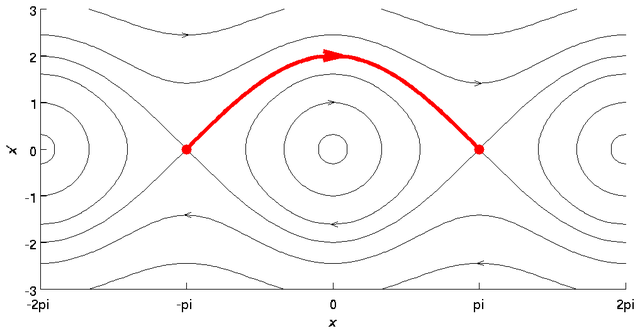
| 解説 | Phaseportrait for the pendulum equation with the heteroclinic orbit highlighted. Created by Jitse Niesen using Matlab. |
| 日付 | 2006年6月29日 (当初のアップロード日) |
| 原典 | コンピュータが読み取れる情報は提供されていませんが、投稿者自身による著作物だと推定されます(著作権の主張に基づく) |
| 作者 | コンピュータが読み取れる情報は提供されていませんが、Jitse Niesenだと推定されます(著作権の主張に基づく) |
Discussion
How come the orbit isn't called homoclinic? The domain is periodic: starting and ending point are the same.
- That depends on what you consider as the domain. If the domain is a circle (and hence periodic), which is the most natural choice, then you're right and the orbit is homoclinic. If the domain is R, the set of real numbers, then the starting and ending point are not the same. But you certainly have a point that this is a confusing example; thanks for that. -- Jitse Niesen 06:45, 2 February 2007 (UTC)
ライセンス
| この著作物の著作権者である私は、この著作物における権利を放棄しパブリックドメインとします。これは全世界で適用されます。 一部の国では、これが法的に可能ではない場合があります。その場合は、次のように宣言します。 私は、あらゆる人に対して、法により必要とされている条件を除き、如何なる条件も課すことなく、あらゆる目的のためにこの著作物を使用する権利を与えます。 |
Matlab source
clf;
axis([-2*pi 2*pi -3 3]);
daspect([1 1 1]);
hold on;

% Draw constant energy contours
qs = linspace(-2*pi, 2*pi, 101);
[Q,P] = meshgrid(qs, linspace(-3,3));
H = P.*P/2 - cos(Q);
contour(Q,P,H, [-0.95 -0.5 0.3  2 4], 'k');

% Draw energy = 0 contour
ps = sqrt(2+2*cos(qs));
plot(qs,ps, 'k');
plot(qs,-ps, 'k');

% Draw heteroclinic connection
qs = linspace(-pi, pi, 101);
ps = sqrt(2+2*cos(qs));
plot(qs,ps, 'r', 'LineWidth', 3);
plot([-pi pi], [0 0], 'r.', 'MarkerSize', 25);

% Arrows
plot(-pi+[-0.10 0.05], sqrt(6)+[0.05 0], 'k');
plot(-pi+[-0.10 0.05], sqrt(6)+[-0.05 0], 'k');
plot(pi+[-0.10 0.05], sqrt(2)+[0.05 0], 'k');
plot(pi+[-0.10 0.05], sqrt(2)+[-0.05 0], 'k');
plot([-0.10 0.05], [1.05 1], 'k');
plot([-0.10 0.05], [0.95 1], 'k');
plot([0.10 -0.05], -sqrt(2.6)+[0.05 0], 'k');
plot([0.10 -0.05], -sqrt(2.6)+[-0.05 0], 'k');
plot(-pi+[0.10 -0.05], -sqrt(2)+[0.05 0], 'k');
plot(-pi+[0.10 -0.05], -sqrt(2)+[-0.05 0], 'k');
plot(pi+[0.10 -0.05], -sqrt(6)+[0.05 0], 'k');
plot(pi+[0.10 -0.05], -sqrt(6)+[-0.05 0], 'k');
plot([-0.2 0.2], [2.1 2], 'r', 'LineWidth', 3);
plot([-0.2 0.2], [1.9 2], 'r', 'LineWidth', 3);

% Axes
xlabel('\it{x}');
ylabel('\it{x}''');
set(gca, 'XTick', [-2*pi -pi 0 pi 2*pi]);
set(gca, 'XTickLabel', {'-2pi' '-pi' '0' 'pi' '2pi'});

% Print
print -dpng 'heteroclinic_tmp.png';
system('convert -trim -bordercolor white -border 10 +repage heteroclinic_tmp.png heteroclinic.png');
ファイルの履歴
過去の版のファイルを表示するには、その版の日時をクリックしてください。
| 日付と時刻 | サムネイル | 寸法 | 利用者 | コメント | |
|---|---|---|---|---|---|
| 現在の版 | 2006年6月29日 (木) 10:50 | | 1,017 × 529 (15キロバイト) | Jitse Niesen | Phaseportrait for the pendulum equation with the heteroclinic orbit highlighted. Created by ~~~ using Matlab. |
ファイルの使用状況
以下のページがこのファイルを使用しています:
グローバルなファイル使用状況
以下に挙げる他のウィキがこの画像を使っています:
- de.wikipedia.org での使用状況
- en.wikipedia.org での使用状況
- en.wikibooks.org での使用状況
- eo.wikipedia.org での使用状況
- it.wikipedia.org での使用状況